Modeling Eddy Currents: Beyond the RL Circuit
Modeling loudspeaker impedance beyond a few hundred Hz is a classic challenge in acoustic engineering. While basic resistance () and inductance () suffice for the low end, eddy current losses in the pole pieces transform the response into a complex system with memory, rendering simple models obsolete.
1. The Legacy: Cauer Networks and Empirical Limits
Traditionally, the industry relies on the Cauer model (). By stacking rungs in a ladder, we attempt to approximate the frequency-dependent nature of magnetic diffusion through an electrical analogy.
While this remains the standard, it hits two major obstacles when seeking high precision:
- Numerical Stiffness: As one attempts to cover more decades of bandwidth, the system becomes mathematically “stiff”, making time-domain simulations either unstable or incredibly slow.
- Lack of Localization: There is no direct spatial correspondence between the network components and the physical iron. The link with physics is broken, making any adjustment for magnetic saturation purely empirical and disconnected from the actual geometry.
2. Mathematical Elegance: Fractional Derivatives
To address the limitations of Cauer networks, using a fractional impedance (where ) offers a seductive alternative. It captures the “semi-inductive” slope with remarkable parameter economy. The Grünwald-Letnikov (GL) formulation allows this concept to be translated into a weighted sum, acting as a long-memory FIR filter.
The Podlubny Approach
To calculate the filter weights , the method described by Podlubny (1999) using an IFFT is the gold standard. By manipulating the generating function , we extract coefficients with high numerical efficiency, even for higher-order approximations.
% FIR weight calculation via IFFT (Munroe Method)
% Extract from PhD Thesis Appendix
nPoints = 1024;
theta = linspace(0, 2*pi, nPoints);
z = exp(-1i * theta);
alpha = 0.5; % Fractional derivative order

% First order approximation (Euler)
% f2 and f3 for higher orders can also be substituted here
f = (1 - z).^alpha;

% Transform to time domain to extract weights
F = real(ifft(f));
nMemory = 512; % FIR filter length
w = F(1:nMemory);
The Computational Wall
However, this elegance quickly hits a wall in real-time applications. To maintain a history of just 1 second at a 96 kHz sampling rate, the processor must handle 96,000 multiplications per sample.
The problem becomes critical during voice coil motion: as the coil moves (), the fractional order changes. Recalculating tens of thousands of coefficients via IFFT at every sample period is computationally impossible for even the most powerful standard DSPs. We have reached a limit: the model simulates the behavior but ignores the structure.
3. The Physical Solution: Method of Lines (MoL)
To break through this wall, Munroe Research utilizes the Method of Lines (MoL). Here, we no longer seek to mimic a curve; instead, we discretize Maxwell’s equations directly within the geometry. For an axisymmetric pole piece, the system input is the axial magnetic field generated by the coil, which diffuses radially () into the material according to:
From PDE to FPGA Implementation
By slicing the radius of the pole into concentric rings, we transform this Partial Differential Equation (PDE) into a system of Ordinary Differential Equations (ODEs).
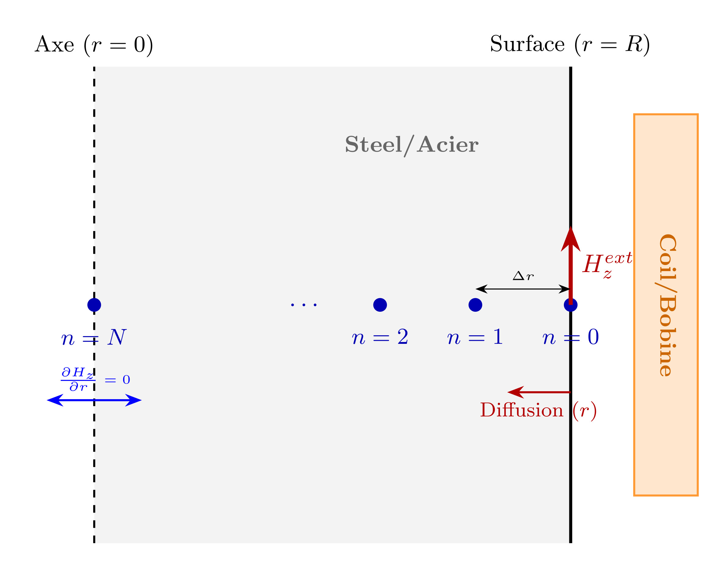
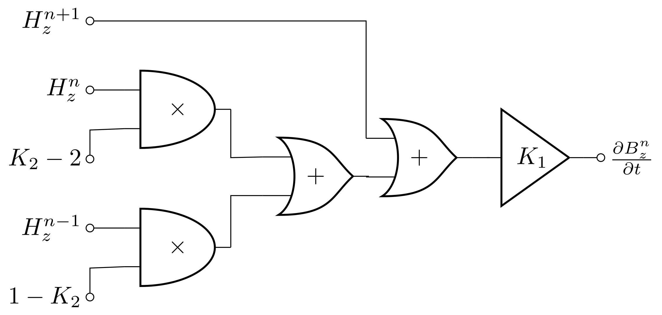
Using a central difference scheme, the diffusion equation is discretized for each point along the radius:
By grouping terms, we obtain an iterative calculation structure perfectly suited for hardware:
The flux is injected at the outer surface (). At the central axis (, or ), we apply a symmetry boundary condition (zero derivative) to ensure the physical continuity of the flux.
High-Performance Kintex-7 Architecture
To achieve real-time execution at 96 kHz, we designed an architecture on a Kintex-7 FPGA using time-division multiplexing. This approach allows us to simulate 128 spatial points in parallel with optimal resource efficiency—a task where a sequential processor would collapse.
Why This Revolutionizes Control
Unlike previous approaches, MoL is a “White Box” model. On the Kintex-7, we have real-time access to the flux density () at every point within the iron. This allows us to natively inject local hysteresis and saturation models. If the pole tip saturates, the model reacts instantly, providing transducer control with unparalleled precision rooted in fundamental physics.
Comparative Summary
| Method | Physical Fidelity | Computational Efficiency | Non-linearities |
|---|---|---|---|
| Cauer | Medium | High (Fixed) | Difficult (Empirical) |
| Fractional | High | Extremely Low | Prohibitive in motion |
| Method of Lines | Excellent | Optimized (Kintex-7) | Native (Physics) |
Conclusion
The Method of Lines on FPGA represents the future of high-precision transducer engineering. By replacing analogies with direct physical simulation, we eliminate the trade-offs between computational complexity and fidelity. More technical details are available in our JAES and IEEE publications listed below.
References and Publications
| Type | Description |
|---|---|
| Book (Theory) | Podlubny, I. “Fractional Differential Equations”, Academic Press, 1999. |
| Journal (IEEE I2MTC) | Munroe, O., et al. “Real-Time FPGA Estimation of Eddy Currents and Hysteresis in Axisymmetric Inductors”, IEEE I2MTC 2025. DOI:10.1109/I2MTC62753.2025.11079216 |
| Journal (JAES) | Munroe, O., et al. “Modeling The Effect Of Eddy Currents On The Inductance Of Loudspeaker Motors Using The Method Of Lines”, JAES 2025. DOI:10.17743/jaes.2022.0188 |